The RRTM model simulates the flow of electromagnetic radiation in and out of the Earth. The orange, red, and purple pairs of arrows on the right represent, respectively, the amount of shortwave radiation (incoming and reflected sunlight), longwave radiation (radiation given off by the ground and atmosphere), and total radiation averaged across the entire Earth's surface. The arrows are graphed as a function of altitude, with the size of the arrow at a given altitude representing the amount of energy being carried per second in that direction per unit area. The size of the arrows is determined by the characteristics of the sun, surface, and atmosphere, which you can manipulate in the control panel on the left. The overall balance of this energy at the top of the atmosphere indicates whether the Earth is gaining energy (and likely warming as a result) or losing energy (and likely cooling).
Inputs
The inputs to the model (the characteristics of the sun, surface, and atmosphere) can be manipulated using the controls in the panel on the left. We'll go tab by tab:
Sun
There's only one value in this tab: the direct sunlight. The direct sunlight is the amount of energy per square meter that would be received each second by a body directly perpendicular to the direction of sunlight. The default value is 1370 W/m2. Keep in mind that the flows in the ouputs are calculated as averages taken over the Earth's surface, so the incoming sunlight as seen in the flows will be only one fourth this value.
Surface
Similarly, there's only one quantity to change in this panel, the albedo. The albedo (α) is the fraction of the sun's radiation that the surface reflects; further, 1 - α is the fraction that the surface absorbs. A value of 1 would indicate that the Earth's surface was a perfect mirror, and therefore absorbs nothing. Conversely, a value of 0 indicates that the Earth's surface is a perfect absorber, and reflects nothing.
You can change the value of the albedo by selecting different surface types, or you can use the slider to manually select a reflectivity.
The default value given is the Earth's average albedo, 0.3; however, the actual average albedo of the surface is much smaller than this, being closer to ~0.1, the albedo of the ocean. Clouds and scattering by the atmosphere make up the difference. The 0.3 value is given to allow for comparison with standard calculations using σ T4.
Atmosphere
This panel allows you to alter properties of the model's atmosphere. Some can be altered directly from the panel, while others must be altered on the graphs that show up when you click on the checkboxes.
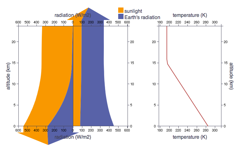
The temperature is assumed by default to be the same throughout the atmosphere. You can see this by clicking on the temperature checkbox. This will show a graph of temperature vs. altitude given in Kelvins. Typically, the atmosphere consists of a number of discrete layers, of which the two most radiatively important are the troposphere (starting at the surface and extending up to the tropopause) and the stratosphere, which starts at the tropopause and extends up further. The troposphere is characterized by a gradual decrease in temperature as one ascends (think of the coldness encountered as one climbs a mountain); the rate of this decrease is known as the lapse rate. The stratopshere is typically more uniform in intemperature, and can even show a slight increase of temperature with height.
You can alter the vertical structure of the atmosphere by changing the lapse rate slider and the tropospheric height slider. 10 K/km is a lapse rate typical of a dry column of atmosphere, while 5 K/km is typical of a saturated column. You can change the surface temperature by dragging on the red circle at the bottom of the graph of temperature. A tooltip should appear indicating the exact value.
You can alter the CO2 (carbon dioxide) or CH4 (methane) concentrations of the atmosphere by clicking on the associated checkboxes to reveal the graph (you might have to scroll over if you already have temperature showing), and then dragging on the red circle at the bottom of the graph.
You can alter the cloudiness by dragging on the sliders for stratus clouds (~1 km high) and cirrus clouds (at the tropospheric height), where the percentages are of cloud cover. You can see the fraction of cloud cover by clicking on the cloud fraction checkbox. You can also alter the cloud water drop radius, one of the parameters used by the model to indicate the clouds' radiatve properties, by clicking on the associated checkbox and dragging the red circle below.
The rest of the controls deal with atmospheric aerosols, aka dust. The dropdown that says "select aerosol profile" contains a number of hypothetical scenarios, for which there are associated vertical profiles of different types of aerosols: sulfates, organic aerosols, black carbon, sea salt, and more. For the four aerosols with checkboxes, you can see the number density (the number of particles per unit volume, in this case meters cubed) of the different aerosols as a function of height.
Outputs
The orange, red, and purple pairs of arrows on the right represent, respectively, the amount of shortwave radiation (incoming and reflected sunlight), longwave radiation (radiation given off by the ground and atmosphere), and total radiation, averaged across the entire Earth's surface. The arrows are graphed as a function of altitude, with the size of the arrow at a given altitude representing the amount of energy being carried per second in that direction, per unit area. You can get the exact value of an arrow at a given altitude by hovering on the arrow.
| Model the full-spectrum (visible + IR) impact of clouds. |
| See the importance of the albedo by changing the Surface condition to snow or ice. |
| See how the lapse rate affects the greenhouse effect. |
| Simulate solar radiation management geoengineering by adding reflective aerosols. |
| Find the model's climate sensitivity. |