The GEOCARB model is based on the Geocarb model for the geologic carbon cycle developed by Robert Berner at Yale. CO₂ is released to the atmosphere as volcanic degassing, and consumed by chemical weathering of rocks on land. These dynamics generate a stabilizing negative feedback called the weathering CO₂ feedback, which stabilizes atmospheric CO₂, and hence Earth's climate, on times scales of hundreds of thousands of years.

This derivative model adds to Berner's original the dynamics of ocean acidification and CaCO₃ neutralization of a CO₂ pulse, which should improve the simulation on time scales of decades to centuries.

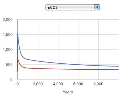
Model atmospheric pCO₂ concentrations after 1,000 and 3,000 Gton C spikes, showing the "long tail" as the persistent increase in pCO₂ after the spike.

The GEOCARB model runs in two basic stages, in initial Spinup stage, then a transition to a Simulation stage at Year 0. The plot only shows the last few years of the Spinup stage, after it has run for long enough to reach equilibrium for the Spinup condtions. You can change model parameters of the CO₂ degassing rate (the flux of CO₂ from the solid Earth to the atmosphere), the existance of land plants, and the relative land areas. If one of these parameters changes between the Spinup and the Simulation stages, the values in the plots before year 0 will show the equilibrium for the Spinup conditions, followed by the transient evolution toward equilibrium for the Simulation stage of the run.

You have the option of releasing a Spike of CO₂ to the atmosphere at the instant of the transition from the Spinup to the Simulation stages. For the default case when the model loads, there is a 1000 Gton C release at the transition, while the driving parameters for the two stages, like CO₂ degassing rates, are the same. You have to expand the time view by selecting Show 1 million years before you can see the carbon cycle return to its equilibrium.

The Silicate thermostat plot shows the weathering rate of CO₂ uptake and the CO₂ degassing rates, both in units of 10¹² moles / year. The CaCO₃ budget plot shows CaCO₃ weathering and burial rates in the ocean, in 10¹² moles / year. There are also plots of ocean chemistry (the alkalinity and total CO₂ concentrations, in mole equivalents / m³, and the carbon isotopic composition of dissolved carbon in the ocean on the PDB scale, labeled del13C) and ocean and atmosphere temperatures.

You can compare two model runs by running the first, then selecting Save This Run to Background. The run will be saved on the plot, and you can superimpose a second by changing model options. Get rid of the backround plot by Deleting it.

How long does it take for a CO2 spike to decay away completely? Which chemical balance or process determines this time scale?

Make a plot of the weathering rate as a function of atmospheric CO2 by setting the volcanic degassing flux to different values and running to equilibrium.

Vary the geologic time to see how the intensity of the sun changes the model behavior.

Introduce plants, keeping everything else constant, to see whether plants make it warm or cool when they appear. Where does the carbon go or come from, to change the atmospheric value?

The University of Chicago 5801 South Ellis Ave Chicago IL 60637 773.702.1234